ro producer’s guide to digital audio

The Pro Producer’s Guide To

If you want to achieve the best mixed and mastered tracks within your DAW, an understanding of how digital audio works is essential. Let’s find out exactly what’s going on ‘inside the box’ as we go back to first principles

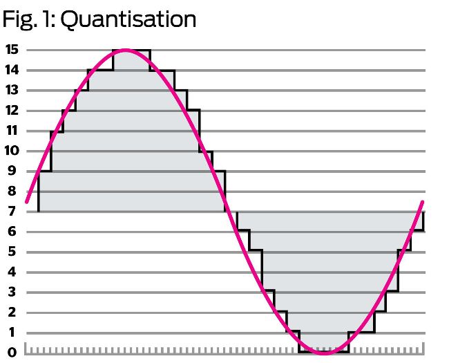
The smooth sine curve is the original analogue waveform; the squared version is the quantised digital waveform

It’s entirely possible to make music on a computer without having the faintest idea of how digital audio works, but a little knowledge can go a long way when it comes to pushing the medium to its limits.

For those unfamiliar with the basics of how sound works, let’s start at square one. Some of the following explanations might seem a little abstract out of the context of actual mixing, but introducing these ideas now is important, as they’ll be referenced when we get more handson later in the issue.

Sound is the oscillation (that is, waves) of pressure through a medium – air, for example. When these waves hit our tympanic membranes (eardrums), the air vibration is converted to a vibration in the fluid that fills the channels of the inner ear. These channels also host cells with microscopic ‘hairs’ (called stereocilia) that release chemical neurotransmitters when pushed hard enough by the vibrations in the fluid. It’s these neurotransmitters that tell our brain what we’re listening to.

The process of recording audio works by converting the pressure waves in the air into an electrical signal. For example, when we (used to) record using a microphone feeding into a tape recorder, the transducer in the mic converts the pressure oscillation in the air into an electrical signal, which is fed to the tape head, which polarises the magnetic particles on the tape running over it in direct proportion to the signal. The movement of sound through air – and, indeed, the signal recorded to tape – is what we’d call an analogue signal. That means that it’s continuous – it moves smoothly from one ‘value’ to the next without ‘stepping’, even under the most microscopic of scrutiny.

By the numbers

Computers are, for the most part, digital, which means they read and write information as discrete values – that is, a string of numbers. So, how do computers turn a smooth waveform of infinite resolution into a series of numbers that they can understand?

The answer is a method called pulse code modulation (PCM), which is the main system employed when working with digital audio information. It starts with the process of analogue-to-digital conversion (ADC), which involves measuring the value of the continuous signal at regular intervals and creating a facsimile of the original waveform. The higher the frequency at which the signal is referenced – or ‘sampled’ – and the greater the precision of the value that’s recorded, the closer to the original waveform the digital recording will be (see Fig. 1).

The number of samples taken per second is called the sampling rate. CD-quality audio is at a sampling rate of 44.1kHz, meaning that the audio signal is sampled a whopping 44,100 times per second. This gives us a pretty smooth representation of even high frequencies – the higher the frequency we want to measure accurately, the higher the sampling rate required. That figure – 44.1kHz – is pretty specific, and there’s a reason for that: the highest frequency that can be represented by PCM audio is exactly half of the sample rate, and the human ear can hear frequencies from around 20Hz to 20kHz, so at the top end that’s 20,000 oscillations (or cycles) per second. This is where we encounter the Nyquist–Shannon sampling theorem, which deals with how often a sample of a signal needs to be taken for it to be reconstructed accurately. The theorem states that the sampling rate needs to be double the highest frequency, lest what’s known as aliasing occurs (see Fig. 2). Aliasing causes unmusical artefacts in the sound, as frequencies higher than the sample rate will be “reflected” around the Nyquist frequency, which is half the sample rate. So at 44.1kHz, Nyquist is 22,050Hz, and if we try to sample, say, 25,050Hz (22,050Hz plus 3000Hz), we’ll instead get 19,050Hz (22,050Hz minus 3000Hz). As frequencies above 20kHz or so can’t be perceived by the human ear, they’re not massively useful anyway.