FALSTAD

Today, computers are nearly always digital, but analogue computers also had their place, as Mike Bedford discovers through emulation.

Credit: www.falstad.com

OUR EXPERT Mike Bedford is interested in both software and hardware, so recreating analogue computers is an ideal excursion for him.

We’re in two minds as to whether debugging a patching error is more difficult than spotting a typo in digital code, but it certainly requires a different mindset.

From the pioneering machines of the ’40s to the home computers of the ’80s, we’ve put F some fascinating computers through their paces via emulation in LXF. But they were all digital, and this ignores an important part of computing’s heritage. The electronic analogue computer was important for scientific applications until the early ’80s. To give these intriguing computers the recognition they deserve, we’re turning to emulation to reveal their secrets.

In this first of two articles, we emulate a very simple machine, then move on to a more sophisticated one next month. We’re not looking at a specific analogue computer, though – we’re emulating a generic one, as models didn’t differ as much as in the digital world. So, forget about bits and logic gates, and get your hands dirty with voltages and operational amplifiers.

Digital vs analogue

Digital and analogue computers differ in two main respects. First, the former represents values that differ in discrete steps, while the latter’s values vary continuously. Second, in digital computers, changes only occur at specific times related to the clock, but in analogue computers, changes happen continuously.

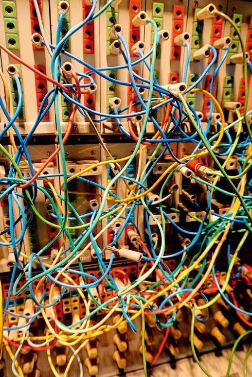
These aren’t the only differences, though, and most importantly, the concept of programming is very different. There’s no such thing as an instruction, so a program isn’t a sequential list of instructions. Instead, it’s a definition of how the analogue computer’s functional units are configured and connected together. Physically, this takes the form of adjusting the value of potentiometers and plugging patch leads into a patch panel.

Analogue and digital computers coexisted for several decades, and we might wonder why, since history rather suggests that digital technology won because it was superior. The answer is tied up with analogue computer applications. Unlike digital computers, analogue machines aren’t universal – they can’t solve all computable problems. Their particular niche – albeit a very important one – is solving sets of differential equations, as required for simulation exercises in science, maths and engineering. On digital computers, this is computationally intensive, as evidenced by the hugely expensive supercomputers used for this sort of application today.

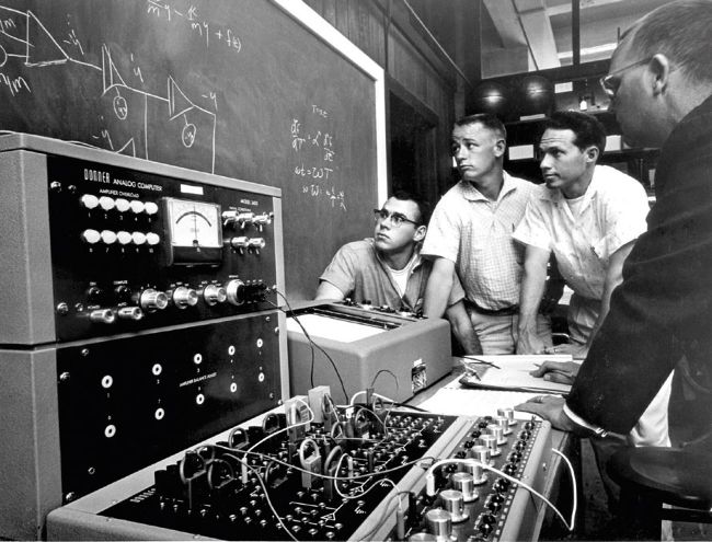
In contrast to the large analogue computers used in industry, desktop machines, like this one from the ’60s, were used in education.

With the digital computers of the ’50s, ’60s and ’70s, this could be a show-stopper, but analogue computers were much quicker. What’s more, the time taken to solve a problem doesn’t increase with the number of equations, a far cry from the situation with digital computers. It wasn’t all one way, though, because analogue computers had drawbacks, too. Programming was often more time consuming, and accuracy was limited because of electrical noise. As a result, digital computers gained the upper hand as their performance improved, even though analogue computers clung on until the early ’80s for the most demanding applications.