SCIL AB

In our continuing journey into analogue computing, Mike Bedford looks at another emulation approach, and how to get a real analogue computer.

As we saw last month, although analogue computers might seem ancient, they gave digital computers a run for their money until the early ’80s. Their particular strength was solving differential equations, so they were used for simulation, primarily in scientific and technical applications.

In the first part of our exposé of electronic analogue computers, we turned to emulation to see how they worked and how they were used. Specifically, we emulated a simple analogue machine – not too dissimilar from the ones that were used in education – but that approach limited the types of problem that could be solved. So, now we’re going to see how to emulate a more sophisticated machine, to allow us to use analogue techniques to solve some more complicated and more interesting problems.

And finally, for those who want to try out some real analogue hardware, as opposed to emulating analogue computers digitally, we’ll introduce some exercises to help you better understand the underlying electronics, and even point you towards a real open hardware machine that you can buy.

A different approach

The emulator that we used last month was built using the Falstad circuit simulator, and this served to provide some insight into analogue computing hardware. The same approach could have been extended to create a larger machine with more potentiometers, summers and integrators. But while this would have allowed problems involving more differential equations to be solved, it would still have been limited. In particular, while it allowed a variable to be multiplied by a constant – this being the function of a potentiometer – it couldn’t multiply two variables. And while lots of problems, like the examples in part one, don’t need a multiplier, many others do. We could have used Falstad to add a multiplier, but while the circuits for potentiometers, summers and integrators are pretty simple, the same isn’t true of an analogue multiplier. If you’re really keen, you could research the subject and try expanding our Falstad-based emulator, but we’re going to pursue a different and simpler way forward.

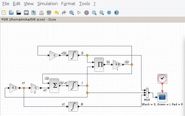
The Susceptible – Infected – Recovered model of an infectious disease, implemented in Xcos, requires multiplication, which wasn’t available in last month’s Falstad emulator.

Our approach maintains the concept of programming by connecting various functional units together – after all, nothing less can be considered as emulating the analogue computing paradigm – but we are making some changes. Most fundamentally, having emulated an analogue computer’s patch panel last month, we’re abandoning that here. Instead, we’re wiring functional blocks together on screen to produce something that looks closer to the wiring diagrams that define how a problem is solved. Essentially, therefore, it eliminates the need to figure out the patching from the wiring diagram, but that’s not really fundamental to the analogue approach.